Module 1: The Exposome — Motivation, Biology, and NHANES
Conducting Exposome-Wide Association Studies
Welcome to the Course
Conducting Exposome-Wide Association Studies (ExWAS)
- 7-module online course
- Learn the statistics and biology behind ExWAS
- Hands-on R programming with real NHANES data
- Culminates in running and interpreting your own ExWAS
Course Overview
| Module | Topic |
|---|---|
| 1 | The Exposome: Motivation, Biology, and NHANES |
| 2 | R and Tidyverse Foundations |
| 3 | Statistical Foundations for ExWAS |
| 4 | The nhanespewas Package |
| 5 | Conducting an ExWAS |
| 6 | Interpreting ExWAS Results |
| 7 | Advanced Topics |
What is the Exposome?
“The exposome encompasses the totality of human environmental exposures from conception onwards, complementing the genome.”
— Christopher Wild, 2005
- The genome is the complete set of DNA
- The exposome is the complete set of environmental exposures
- Together, they shape health and disease
The E-G-P-D Framework
Our conceptual model links:
- Environment (exposures): chemicals, nutrients, pollutants, lifestyle
- Genome: inherited genetic variation
- Phenotype: measurable traits (BMI, glucose, blood pressure)
- Disease: clinical outcomes (T2D, cardiovascular disease)
\[E + G \rightarrow P \rightarrow D\]
Understanding the exposome means understanding E in this framework.
Why Study the Exposome?
The rise of chronic disease:
- Type 2 diabetes prevalence has increased dramatically over the past 40 years
- Obesity rates have tripled since the 1970s
- Genetics alone cannot explain these rapid changes
- Environmental factors — diet, chemicals, lifestyle — are key drivers
CDC Diabetes Atlas: https://www.cdc.gov/diabetes/php/data-research/index.html
Genetic vs. Environmental Contributions
- Genome-Wide Association Studies (GWAS) have identified hundreds of loci for complex traits
- Yet GWAS variants typically explain <20% of trait heritability
- The “missing heritability” problem suggests environmental factors play a large role
- ExWAS is the environmental analogue of GWAS
What is an ExWAS?
Exposome-Wide Association Study (ExWAS):
- Systematically test associations between many environmental exposures and a health outcome
- Analogous to GWAS: instead of scanning SNPs, scan exposures
- Data-driven, hypothesis-generating approach
First described in: Patel et al. 2010, PLoS ONE
ExWAS: The Concept
- Measure a large panel of environmental exposures (E₁, E₂, …, Eₘ)
- Measure a phenotype or disease outcome (P or D)
- Test each exposure-phenotype association individually
- Correct for multiple testing
- Replicate findings in independent data
The National Health and Nutrition Examination Survey (NHANES)
- Conducted by the US CDC / National Center for Health Statistics (NCHS)
- Representative sample of the non-institutionalized US population
- Continuous since 1999, released in 2-year cycles
- Combines interviews, physical examinations, and laboratory tests
https://www.cdc.gov/nchs/nhanes/index.htm
Why NHANES for ExWAS?
- Hundreds of environmental biomarkers measured in blood and urine
- Linked to health phenotypes (BMI, glucose, lipids, blood pressure)
- Demographic and socioeconomic data available
- Survey weights enable nationally representative estimates
- Publicly available and well-documented
NHANES Sampling Design
NHANES uses a complex, multi-stage probability sampling design:
- Primary Sampling Units (PSUs): counties or groups of counties
- Strata: geographic/demographic divisions within PSUs
- Households: selected within strata
- Individuals: selected within households
This design requires special statistical methods (Module 3).
NHANES Survey Cycles
| Cycle | Years | Key Variables |
|---|---|---|
| 1 | 1999-2000 | Core demographics, lab biomarkers |
| 2 | 2001-2002 | Expanded environmental panel |
| 3 | 2003-2004 | Continued monitoring |
| 4 | 2005-2006 | Additional pollutants |
| … | … | Ongoing |
Our training data uses cycles 1-2; testing data uses cycles 3-4.
Types of Exposures in NHANES
Biomarkers of environmental exposure:
- Metals: lead (Pb), cadmium (Cd), mercury (Hg)
- Persistent organic pollutants: PCBs, dioxins, pesticides
- Volatile organic compounds: benzene metabolites
- Nutrients: vitamins, minerals, fatty acids
- Lifestyle: cotinine (smoking), caffeine
Measured in blood and urine samples.
Let’s Load Our Data
This .Rdata file contains:
NHData.train: training dataset (NHANES 1999-2002)NHData.test: testing dataset (NHANES 2003-2006)ExposureList: array of exposure variable namesExposureDescription: dictionary of exposure variablesdemographicVariables: dictionary of demographic variables
Exploring the Training Data
We have 21004 individuals and 193 variables in the training set.
How Many Exposures?
We have 160 environmental exposures to test.
Exposure Descriptions
| tab_name | tab_desc | series | module | var | var_desc | tab_desc_ewas | analyzable | var_desc_ewas | binary_ref_group | var_desc_ewas_sub | comment_var | version_date | is_comment | is_weight | is_questionnaire | is_ecological | is_binary | is_ordinal | categorical_ref_group | categorical_levels | |
|---|---|---|---|---|---|---|---|---|---|---|---|---|---|---|---|---|---|---|---|---|---|
| 52 | l06bmt_c | Blood Lead, Cadmium, Mercury | 2003-2004 | laboratory | LBXBCD | Cadmium (ug/L) | heavy metals | 1 | heavy metals | NA | NA | NA | 2009-11-13 | 0 | 0 | 0 | 0 | 0 | NA | NA | NA |
| 54 | l06bmt_c | Blood Lead, Cadmium, Mercury | 2003-2004 | laboratory | LBXBPB | Lead (ug/dL) | heavy metals | 1 | heavy metals | NA | NA | NA | 2009-11-13 | 0 | 0 | 0 | 0 | 0 | NA | NA | NA |
| 56 | l06bmt_c | Blood Lead, Cadmium, Mercury | 2003-2004 | laboratory | LBXTHG | Mercury, total (ug/L) | heavy metals | 1 | heavy metals | NA | NA | NA | 2009-11-13 | 0 | 0 | 0 | 0 | 0 | NA | NA | NA |
| 58 | l06bmt_c | Blood Lead, Cadmium, Mercury | 2003-2004 | laboratory | LBXIHG | Mercury, inorganic (ug/L) | heavy metals | 1 | heavy metals | NA | NA | NA | 2009-11-13 | 0 | 0 | 0 | 0 | 0 | NA | NA | NA |
| 60 | l06cot_c | Cotinine | 2003-2004 | laboratory | LBXCOT | Cotinine (ng/mL) | biochemistry | 1 | cotinine | NA | NA | NA | 2009-11-13 | 0 | 0 | 0 | 0 | 0 | NA | NA | NA |
| 61 | l06hm_c | Heavy Metals | 2003-2004 | laboratory | URXUBA | Barium, urine (ng/mL) | heavy metals | 1 | heavy metals | NA | NA | URDUBALC | 2009-11-13 | 0 | 0 | 0 | 0 | 0 | NA | NA | NA |
| 62 | l06hm_c | Heavy Metals | 2003-2004 | laboratory | URXUBE | Beryllium, urine (ng/mL) | heavy metals | 1 | heavy metals | NA | NA | URDUBELC | 2009-11-13 | 0 | 0 | 0 | 0 | 0 | NA | NA | NA |
| 63 | l06hm_c | Heavy Metals | 2003-2004 | laboratory | URXUCD | Cadmium, urine (ng/mL) | heavy metals | 1 | heavy metals | NA | NA | URDUCDLC | 2009-11-13 | 0 | 0 | 0 | 0 | 0 | NA | NA | NA |
| 64 | l06hm_c | Heavy Metals | 2003-2004 | laboratory | URXUCO | Cobalt, urine (ng/mL) | heavy metals | 1 | heavy metals | NA | NA | URDUCOLC | 2009-11-13 | 0 | 0 | 0 | 0 | 0 | NA | NA | NA |
| 65 | l06hm_c | Heavy Metals | 2003-2004 | laboratory | URXUCS | Cesium, urine (ng/mL) | heavy metals | 1 | heavy metals | NA | NA | URDUCSLC | 2009-11-13 | 0 | 0 | 0 | 0 | 0 | NA | NA | NA |
Key Phenotypes
Our primary phenotypes related to Type 2 Diabetes:
| Variable | Description | Units |
|---|---|---|
BMXBMI |
Body Mass Index | kg/m² |
LBXGLU |
Fasting Blood Glucose | mg/dL |
Demographic Variables
| var | description |
|---|---|
| SEQN | ID |
| RIDAGEYR | age (years) |
| female | female sex |
| male | male sex |
| black | Black |
| mexican | Mexican American |
| other_hispanic | Other Hispanic |
| other_eth | Other Race/Ethnicity |
| SES_LEVEL | SES Tertile (0, 1, 2) |
| education | Education (< HS, =HS, >HS) |
Key Demographic Variables
| Variable | Description |
|---|---|
RIDAGEYR |
Age in years |
male / female |
Sex (binary indicators) |
white, black, mexican, other_hispanic, other_eth |
Race/Ethnicity (binary indicators) |
INDFMPIR |
Income-to-poverty ratio |
SES_LEVEL |
SES tertile (0, 1, 2) |
SDMVPSU |
Primary sampling unit |
SDMVSTRA |
Stratum |
WTMEC2YR |
2-year survey weight |
Variable Types in Our Data
| variable | type |
|---|---|
| BMXBMI | numeric |
| LBXGLU | numeric |
| RIDAGEYR | numeric |
| male | numeric |
| black | numeric |
| INDFMPIR | numeric |
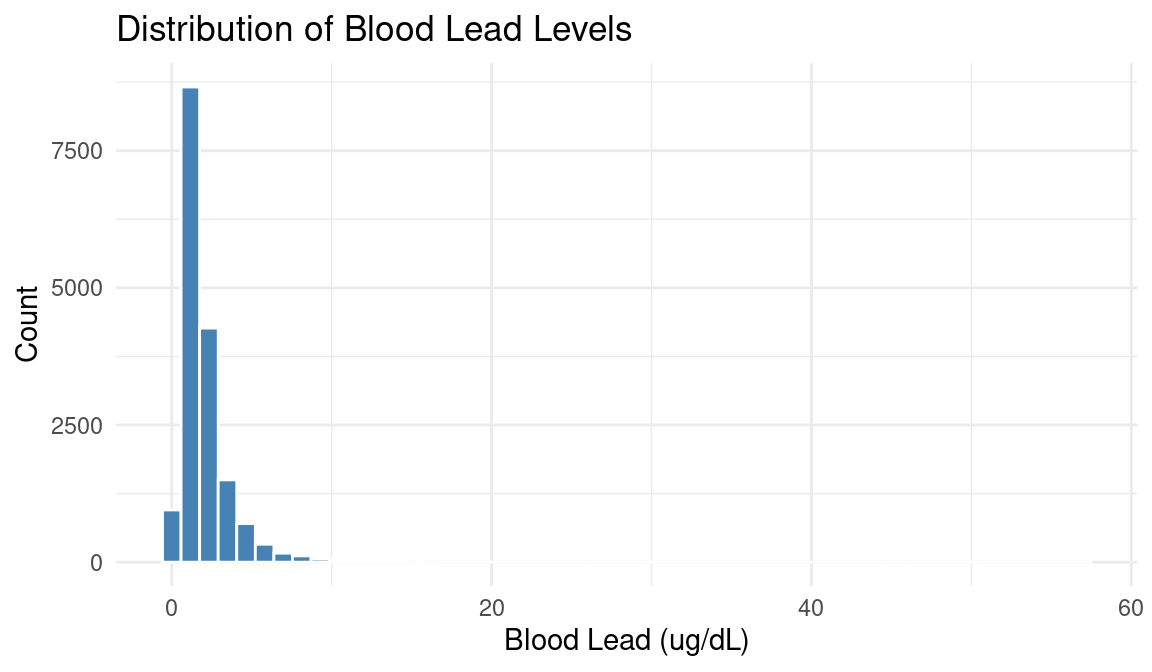
Exploring an Exposure: Blood Lead
Challenges of Exposome Research
- Multiple testing: hundreds of tests inflate false positives
- Correlation among exposures: exposures are not independent
- Confounding: demographic and socioeconomic factors affect both exposure and outcome
- Measurement error: biomarkers are imperfect proxies of true exposure
- Reverse causation: disease may affect exposure levels
- Temporal variability: single time-point measurement
The Multiple Testing Problem
- Testing 160 exposures simultaneously
- At \(\alpha = 0.05\), we expect ~8 false positives by chance
- Solutions:
- Bonferroni correction: \(\alpha / m\) (conservative)
- Benjamini-Hochberg FDR: controls false discovery rate (less conservative)
- More detail in Module 3
Correlation Among Exposures
- Environmental exposures are often correlated
- Smokers have higher cadmium AND lead
- Dietary nutrients co-occur in food patterns
- Pollutants share environmental sources
- Correlated exposures complicate interpretation
- Cannot isolate the “causal” exposure from correlated panel
Confounding
- A confounder is a variable that influences both the exposure and the outcome
- Example: age affects both lead levels (older cohorts had more lead exposure) and BMI
- Must adjust for confounders in regression models
- Common confounders: age, sex, race/ethnicity, socioeconomic status
Key References
- Wild CP. Complementing the genome with an “exposome.” Cancer Epidemiol Biomarkers Prev. 2005.
- Patel CJ, Bhattacharya J, Butte AJ. An Environment-Wide Association Study (EWAS) on Type 2 Diabetes Mellitus. PLoS ONE. 2010.
- Patel CJ, et al. A database of human exposomes and phenomes from the US NHANES. Scientific Data. 2016.
- Chung MK, et al. The exposome and exposome-wide association studies. Exposome. 2024.
What’s Next?
Module 2: R and Tidyverse Foundations
- The pipe operator and dplyr verbs
- Data visualization with ggplot2
- Linear regression with broom
- Building pipelines for many regressions
Summary
- The exposome represents the totality of environmental exposures
- ExWAS systematically scans exposures for associations with health outcomes
- NHANES provides a rich, publicly available dataset for ExWAS
- Key challenges: multiple testing, confounding, correlation, measurement error
- This course will teach you to conduct, interpret, and extend ExWAS analyses
Supported By
This course is supported by the National Institutes of Health (NIH):
- National Institute of Environmental Health Sciences (NIEHS): R01ES032470, U24ES036819
- National Institute of Diabetes and Digestive and Kidney Diseases (NIDDK): R01DK137993