Module 2: R and Tidyverse Foundations

Conducting Exposome-Wide Association Studies

Chirag J Patel

Overview

In this module, we will cover:

1. The pipe operator (%>% and |>)
2. Six core dplyr verbs: filter, select, mutate, arrange, summarize, group_by
3. Recoding variables with case_when
4. Tidy data and reshaping with pivot_longer/pivot_wider
5. Visualization with ggplot2
6. Linear regression in R and the broom package
7. Running many regressions with nest_by

The Tidyverse Ecosystem

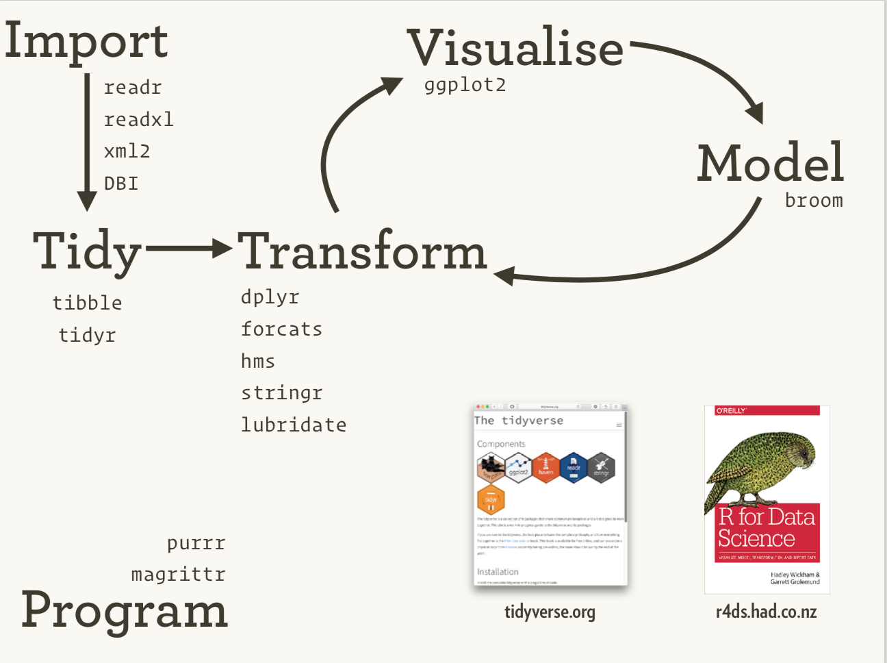
The tidyverse is an ecosystem of R packages for data science, originally conceived by Hadley Wickham.

Our Dataset

We use NHANES data from the training set:

nhData <- NHData.train %>%
  select(BMXBMI, LBXGLU, RIDAGEYR, male, female,
         black, mexican, other_hispanic, other_eth, white,
         SDDSRVYR, LBXBPB, LBXBCD, INDFMPIR) %>%
  mutate(PID = row_number())

nhData %>% sample_n(5) %>%
  select(PID, BMXBMI, LBXGLU, RIDAGEYR, male, black, white) %>%
  kable() %>% kable_styling(font_size = 9)

PID	BMXBMI	LBXGLU	RIDAGEYR	male	black	white
7226	15.26	NA	3	1	0	1
19852	NA	NA	13	0	0	0
1863	16.64	NA	8	0	1	0
20161	16.55	NA	5	1	0	1
3538	25.21	152.7	71	1	1	0

The Pipe Operator

The pipe %>% passes the output of one function as the first argument of the next:

x %>% f(y)   is equivalent to   f(x, y)

Base R also has a native pipe: |>

# Without pipe
head(nhData, n = 3) %>% select(PID, BMXBMI, RIDAGEYR, male)

  PID BMXBMI RIDAGEYR male
1   1  14.90        2    0
2   2  24.90       77    1
3   3  17.63       10    0

# With pipe
nhData %>% head(n = 3) %>% select(PID, BMXBMI, RIDAGEYR, male)

  PID BMXBMI RIDAGEYR male
1   1  14.90        2    0
2   2  24.90       77    1
3   3  17.63       10    0

Why Pipe?

Pipes make code more readable by expressing operations left-to-right:

# Nested (hard to read)
head(arrange(filter(nhData, male == 1), -BMXBMI), 5)

# Piped (easy to read)
nhData %>%
  filter(male == 1) %>%
  arrange(-BMXBMI) %>%
  head(5)

dplyr: Six Core Verbs

Verb	Purpose
filter()	Select rows by conditions
select()	Choose columns
mutate()	Create or modify columns
arrange()	Sort rows
summarize()	Collapse to summary statistics
group_by()	Partition data into groups

filter(): Select Rows

# Filter to males only
nhData %>%
  filter(male == 1) %>%
  select(PID, BMXBMI, LBXGLU, RIDAGEYR, male) %>%
  head(3) %>%
  kable() %>% kable_styling(font_size = 9)

PID	BMXBMI	LBXGLU	RIDAGEYR	male
2	24.9	83.7	77	1
4	NA	NA	1	1
5	29.1	99.9	49	1

filter(): Multiple Conditions

# Males with glucose >= 126 (diabetic range)
nhData %>%
  filter(male == 1, LBXGLU >= 126) %>%
  select(PID, BMXBMI, LBXGLU, RIDAGEYR, male) %>%
  head(5) %>%
  kable() %>% kable_styling(font_size = 9)

PID	BMXBMI	LBXGLU	RIDAGEYR	male
29	36.94	142.1	62	1
211	31.30	133.7	76	1
266	29.51	165.6	82	1
272	22.36	221.2	56	1
695	26.10	166.1	59	1

select(): Choose Columns

# Select specific columns
nhData %>% select(male, BMXBMI) %>% head(5)

# Remove columns
nhData %>% select(-c(PID, SDDSRVYR)) %>% head(5)

# Select by name pattern
nhData %>% select(starts_with("LB")) %>% head(5)

Other helpers: ends_with(), contains(), matches(), one_of()

select(): Example Output

nhData %>%
  select(starts_with("LB")) %>%
  head(5) %>%
  kable() %>% kable_styling(font_size = 9)

LBXGLU	LBXBPB	LBXBCD
NA	NA	NA
83.7	5.0	0.2
NA	2.2	0.2
NA	9.2	0.2
99.9	1.6	0.4

Combining filter and select

nhData %>%
  filter(male == 1, LBXGLU > 100) %>%
  select(BMXBMI, LBXGLU) %>%
  head(5) %>%
  kable() %>% kable_styling()

BMXBMI	LBXGLU
36.94	142.1
29.74	105.9
29.28	106.6
18.43	103.6
30.67	102.9

mutate(): Create New Columns

nhData %>%
  mutate(
    obese = BMXBMI >= 30,
    t2d = LBXGLU >= 126
  ) %>%
  select(BMXBMI, obese, LBXGLU, t2d) %>%
  head(5) %>%
  kable() %>% kable_styling()

BMXBMI	obese	LBXGLU	t2d
14.90	FALSE	NA	NA
24.90	FALSE	83.7	FALSE
17.63	FALSE	NA	NA
NA	NA	NA	NA
29.10	FALSE	99.9	FALSE

case_when(): Recode Variables

case_when works like a switch statement inside mutate:

nhData <- nhData %>%
  mutate(
    gender = case_when(
      male == 1 ~ "Male",
      female == 1 ~ "Female"
    ),
    ethnicity = case_when(
      white == 1 ~ "White",
      black == 1 ~ "Black",
      mexican == 1 ~ "Mexican American",
      other_hispanic == 1 ~ "Other Hispanic",
      other_eth == 1 ~ "Other"
    )
  )

case_when(): Age Groups

nhData <- nhData %>%
  mutate(
    age_group = case_when(
      RIDAGEYR < 18 ~ "[0,18)",
      RIDAGEYR < 30 ~ "[18,30)",
      RIDAGEYR < 60 ~ "[30,60)",
      RIDAGEYR >= 60 ~ "[60+)"
    )
  )

nhData %>%
  count(age_group) %>%
  kable() %>% kable_styling()

age_group	n
[0,18)	9563
[18,30)	3039
[30,60)	4696
[60+)	3706

arrange(): Sort Rows

nhData %>%
  select(BMXBMI, LBXGLU, gender) %>%
  arrange(-LBXGLU) %>%
  head(5) %>%
  kable() %>% kable_styling()

BMXBMI	LBXGLU	gender
24.51	686.2	Male
29.46	587.3	Male
27.55	581.6	Female
31.16	445.0	Male
30.82	442.7	Male

summarize(): Collapse to Summary

nhData %>%
  summarize(
    n = n(),
    mean_bmi = mean(BMXBMI, na.rm = TRUE),
    sd_bmi = sd(BMXBMI, na.rm = TRUE),
    mean_glucose = mean(LBXGLU, na.rm = TRUE)
  ) %>%
  kable(digits = 2) %>% kable_styling()

n	mean_bmi	sd_bmi	mean_glucose
21004	24.79	7.03	100.51

group_by(): Partition Data

nhData %>%
  group_by(gender) %>%
  summarize(
    n = n(),
    mean_bmi = mean(BMXBMI, na.rm = TRUE),
    mean_glucose = mean(LBXGLU, na.rm = TRUE)
  ) %>%
  kable(digits = 2) %>% kable_styling()

gender	n	mean_bmi	mean_glucose
Female	10790	25.21	97.91
Male	10214	24.36	103.29

group_by(): Multiple Groups

nhData %>%
  mutate(obese = BMXBMI >= 30) %>%
  group_by(gender, obese) %>%
  summarize(
    n = n(),
    mean_glucose = mean(LBXGLU, na.rm = TRUE),
    .groups = "drop"
  ) %>%
  kable(digits = 2) %>% kable_styling()

gender	obese	n	mean_glucose
Female	FALSE	6909	94.93
Female	TRUE	2085	105.23
Female	NA	1796	102.56
Male	FALSE	7028	100.74
Male	TRUE	1450	110.94
Male	NA	1736	117.89

Tidy Data

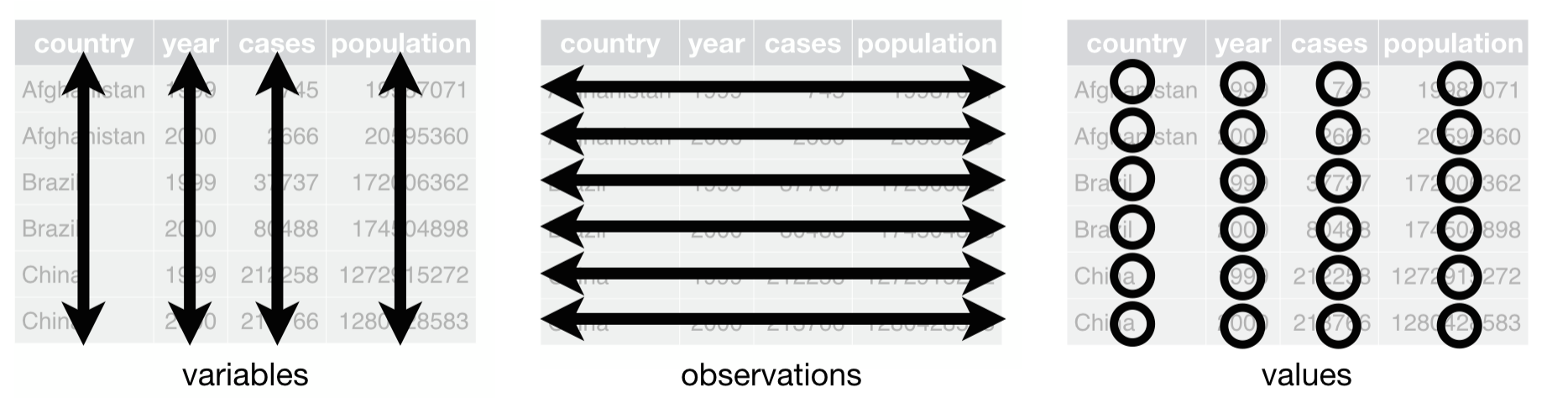
Tidy data principles (Hadley Wickham, inspired by E.F. Codd):

1. Each variable forms a column
2. Each observation forms a row
3. Each type of observational unit forms a table

Is NHANES Tidy?

nhData %>%
  select(PID, BMXBMI, LBXGLU, gender, ethnicity) %>%
  sample_n(5) %>%
  kable() %>% kable_styling()

PID	BMXBMI	LBXGLU	gender	ethnicity
17050	23.57	NA	Male	Mexican American
1954	25.32	94.3	Male	Black
8258	15.77	NA	Male	Other Hispanic
11012	20.98	NA	Female	White
4322	37.97	97.8	Female	White

Yes — each row is one participant’s measurements.

pivot_longer(): Wide to Long

nhData_long <- nhData %>%
  pivot_longer(
    cols = c(BMXBMI, LBXGLU),
    names_to = "measurement",
    values_to = "value"
  )

nhData_long %>%
  select(PID, measurement, value, gender) %>%
  head(6) %>%
  kable() %>% kable_styling()

PID	measurement	value	gender
1	BMXBMI	14.90	Female
1	LBXGLU	NA	Female
2	BMXBMI	24.90	Male
2	LBXGLU	83.70	Male
3	BMXBMI	17.63	Female
3	LBXGLU	NA	Female

pivot_wider(): Long to Wide

nhData_wide <- nhData_long %>%
  select(PID, measurement, value) %>%
  pivot_wider(names_from = measurement, values_from = value)

nhData_wide %>%
  head(5) %>%
  kable() %>% kable_styling()

PID	BMXBMI	LBXGLU
1	14.90	NA
2	24.90	83.7
3	17.63	NA
4	NA	NA
5	29.10	99.9

ggplot2: Grammar of Graphics

Components of a ggplot:

• data: the data frame
• aes(): aesthetic mappings (x, y, color, size, shape)
• geom_*(): geometric objects (points, bars, lines)
• facet_*(): faceting for small multiples
• theme_*(): appearance

ggplot(data, aes(x = var1, y = var2)) +
  geom_point()

Histogram

ggplot(nhData, aes(x = BMXBMI)) +
  geom_histogram(bins = 40, fill = "steelblue", color = "white") +
  labs(x = "BMI (kg/m²)", y = "Count", title = "Distribution of BMI") +
  theme_minimal()

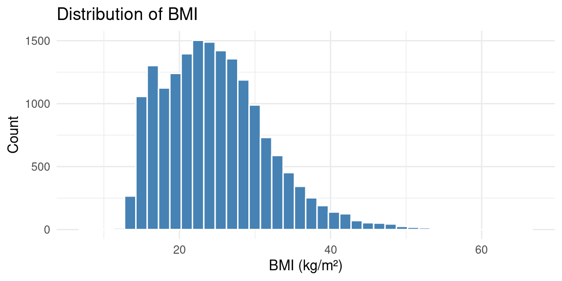
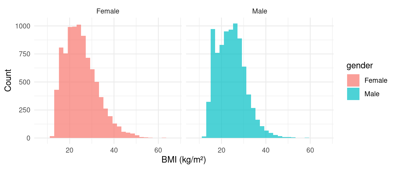
Histogram with Facets

ggplot(nhData, aes(x = BMXBMI, fill = gender)) +
  geom_histogram(bins = 30, alpha = 0.7) +
  facet_wrap(~gender) +
  labs(x = "BMI (kg/m²)", y = "Count") +
  theme_minimal()

Boxplot

ggplot(nhData, aes(x = gender, y = BMXBMI, color = gender)) +
  geom_boxplot() +
  labs(x = "Sex", y = "BMI (kg/m²)", title = "BMI by Sex") +
  theme_minimal()

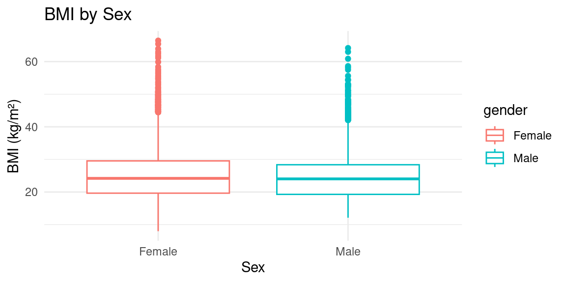
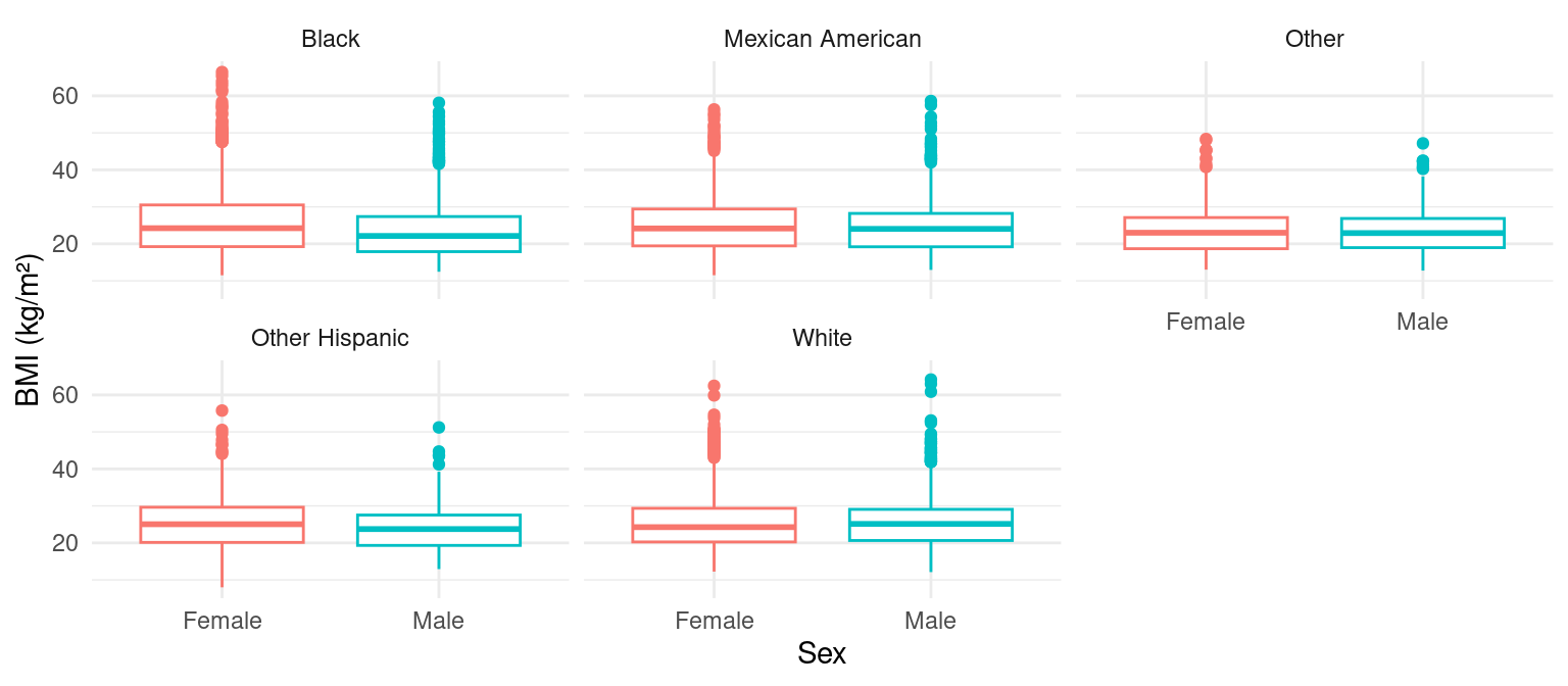
Boxplot with Facets by Ethnicity

ggplot(nhData, aes(x = gender, y = BMXBMI, color = gender)) +
  geom_boxplot() +
  facet_wrap(~ethnicity) +
  labs(x = "Sex", y = "BMI (kg/m²)") +
  theme_minimal() +
  theme(legend.position = "none")

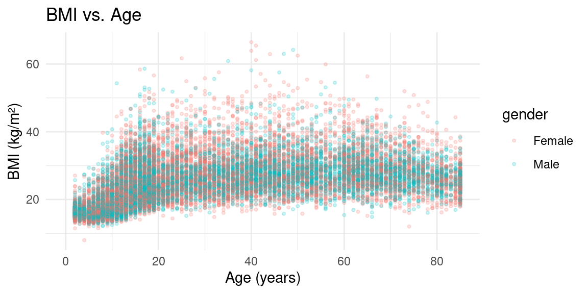
Scatterplot

ggplot(nhData, aes(x = RIDAGEYR, y = BMXBMI, color = gender)) +
  geom_point(alpha = 0.2, size = 0.8) +
  labs(x = "Age (years)", y = "BMI (kg/m²)", title = "BMI vs. Age") +
  theme_minimal()

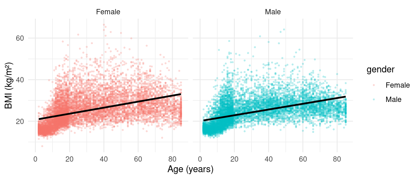
Scatterplot with Facets

ggplot(nhData, aes(x = RIDAGEYR, y = BMXBMI, color = gender)) +
  geom_point(alpha = 0.2, size = 0.5) +
  facet_wrap(~gender) +
  geom_smooth(method = "lm", se = FALSE, color = "black") +
  labs(x = "Age (years)", y = "BMI (kg/m²)") +
  theme_minimal()

Linear Regression in R

Model the relationship: \(y = \alpha + \sum_{i=1}^{M} \beta_i x_i\)

fit <- lm(LBXGLU ~ BMXBMI + RIDAGEYR + male + black + mexican +
            other_hispanic + other_eth,
          data = nhData)

Three levels of output:

1. Model level: \(R^2\), residual standard error
2. Term level: coefficient estimates, p-values
3. Observation level: predictions, residuals

Model Summary

summary(fit)

Call:
lm(formula = LBXGLU ~ BMXBMI + RIDAGEYR + male + black + mexican + 
    other_hispanic + other_eth, data = nhData)

Residuals:
   Min     1Q Median     3Q    Max 
-77.67 -11.76  -4.21   3.49 592.88 

Coefficients:
               Estimate Std. Error t value Pr(>|t|)    
(Intercept)    64.46384    1.80388  35.736  < 2e-16 ***
BMXBMI          0.57673    0.06243   9.237  < 2e-16 ***
RIDAGEYR        0.39515    0.01863  21.212  < 2e-16 ***
male            5.62365    0.76229   7.377 1.82e-13 ***
black           1.98181    1.02949   1.925  0.05427 .  
mexican         5.83894    0.94913   6.152 8.12e-10 ***
other_hispanic  5.56316    1.84842   3.010  0.00263 ** 
other_eth       5.29182    2.15850   2.452  0.01425 *  
---
Signif. codes:  0 '***' 0.001 '**' 0.01 '*' 0.05 '.' 0.1 ' ' 1

Residual standard error: 30.25 on 6324 degrees of freedom
  (14672 observations deleted due to missingness)
Multiple R-squared:  0.1068,    Adjusted R-squared:  0.1058 
F-statistic:   108 on 7 and 6324 DF,  p-value: < 2.2e-16

Interpreting the Coefficients

• BMXBMI: change in glucose per 1 kg/m² increase in BMI
• RIDAGEYR: change in glucose per 1 year increase in age
• male: difference in glucose for males vs. females (reference)
• black, mexican, etc.: difference vs. white (reference group)

Reference categories: female for sex, white for race/ethnicity.

The broom Package

broom tidies model output into data frames:

Function	Returns	Description
glance()	1-row tibble	Model-level summary (\(R^2\), AIC)
tidy()	Per-term tibble	Coefficients, p-values per variable
augment()	Per-observation tibble	Predictions, residuals

glance(): Model-Level Summary

glance(fit) %>%
  select(r.squared, adj.r.squared, sigma, p.value) %>%
  kable(digits = 4) %>% kable_styling()

r.squared	adj.r.squared	sigma	p.value
0.1068	0.1058	30.2453	0

tidy(): Term-Level Summary

tidy(fit) %>%
  select(term, estimate, std.error, p.value) %>%
  kable(digits = 4) %>% kable_styling(font_size = 9)

term	estimate	std.error	p.value
(Intercept)	64.4638	1.8039	0.0000
BMXBMI	0.5767	0.0624	0.0000
RIDAGEYR	0.3952	0.0186	0.0000
male	5.6237	0.7623	0.0000
black	1.9818	1.0295	0.0543
mexican	5.8389	0.9491	0.0000
other_hispanic	5.5632	1.8484	0.0026
other_eth	5.2918	2.1585	0.0142

augment(): Observation-Level

augment(fit) %>%
  select(LBXGLU, .fitted, .resid) %>%
  head(5) %>%
  kable(digits = 2) %>% kable_styling()

LBXGLU	.fitted	.resid
83.7	114.87	-31.17
99.9	106.23	-6.33
85.6	106.71	-21.11
84.2	84.17	0.03
89.8	106.90	-17.10

Running Many Regressions with nest_by

Goal: Predict BMI and glucose as a function of age, sex, ethnicity — stratified by survey year.

Step 1: Make data long

nhData_long <- nhData %>%
  pivot_longer(cols = c(LBXGLU, BMXBMI),
               names_to = "outcome",
               values_to = "value")

Step 2: nest_by and Fit Models

regressions <- nhData_long %>%
  nest_by(outcome, SDDSRVYR) %>%
  mutate(fit = list(lm(value ~ RIDAGEYR + male + black + mexican +
                         other_hispanic + other_eth,
                       data = data))) %>%
  select(-data)

regressions

# A tibble: 4 × 3
# Rowwise:  outcome, SDDSRVYR
  outcome SDDSRVYR fit   
  <chr>      <dbl> <list>
1 BMXBMI         1 <lm>  
2 BMXBMI         2 <lm>  
3 LBXGLU         1 <lm>  
4 LBXGLU         2 <lm>  

Step 3: Extract R² from Each Model

regressions %>%
  summarise(glance(fit)) %>%
  select(outcome, SDDSRVYR, r.squared) %>%
  arrange(outcome, SDDSRVYR) %>%
  kable(digits = 3) %>% kable_styling()

outcome	SDDSRVYR	r.squared
BMXBMI	1	0.228
BMXBMI	2	0.233
LBXGLU	1	0.103
LBXGLU	2	0.090

Step 4: Extract Coefficients from Each Model

regressions %>%
  summarise(tidy(fit)) %>%
  select(outcome, SDDSRVYR, term, estimate, p.value) %>%
  head(10) %>%
  kable(digits = 3) %>% kable_styling(font_size = 9)

outcome	SDDSRVYR	term	estimate	p.value
BMXBMI	1	(Intercept)	20.075	0.000
BMXBMI	1	RIDAGEYR	0.145	0.000
BMXBMI	1	male	-1.063	0.000
BMXBMI	1	black	1.453	0.000
BMXBMI	1	mexican	1.209	0.000
BMXBMI	1	other_hispanic	0.854	0.005
BMXBMI	1	other_eth	0.818	0.028
BMXBMI	2	(Intercept)	19.948	0.000
BMXBMI	2	RIDAGEYR	0.149	0.000
BMXBMI	2	male	-0.632	0.000

Putting It All Together

The tidyverse workflow for ExWAS:

1. Load and clean data with dplyr (mutate, filter, select)
2. Reshape data with tidyr (pivot_longer)
3. Visualize data with ggplot2
4. Model with lm() or svyglm()
5. Tidy results with broom (tidy, glance)
6. Scale analyses with nest_by + map

Summary

• The pipe operator makes code readable and composable
• dplyr provides 6 core verbs for data manipulation
• case_when enables flexible variable recoding
• pivot_longer/wider reshapes data between wide and long formats
• ggplot2 creates publication-quality visualizations
• broom tidies model output for downstream analysis
• nest_by scales regressions across groups

What’s Next?

Module 3: Statistical Foundations for ExWAS

• Survey sampling and svydesign/svyglm
• Log transformation and standardization
• Multiple testing correction
• Confounding and DAGs

Supported By

This course is supported by the National Institutes of Health (NIH):

• National Institute of Environmental Health Sciences (NIEHS): R01ES032470, U24ES036819
• National Institute of Diabetes and Digestive and Kidney Diseases (NIDDK): R01DK137993