Module 3: Statistical Foundations for ExWAS

Conducting Exposome-Wide Association Studies

Chirag J Patel

Overview

This module covers the statistical machinery behind ExWAS:

1. Survey sampling concepts
2. svydesign() and svyglm() vs. lm()
3. Multivariate regression
4. Log transformation of skewed exposures
5. Z-score standardization
6. Multiple testing: Bonferroni vs. FDR
7. Confounding and DAGs
8. R-squared and delta R-squared

Why Special Statistics for NHANES?

NHANES uses complex survey sampling — not simple random sampling:

• Certain subpopulations are oversampled (e.g., minorities, elderly)
• Participants within the same PSU/stratum are correlated
• Each participant has a sampling weight reflecting how many people they represent

Consequence: Standard lm() produces biased standard errors and invalid p-values.

The Survey Package

The survey package in R handles complex survey designs:

library(survey)

Two key functions:

1. svydesign() — declare the survey design
2. svyglm() — fit regression models accounting for the design

Creating a Survey Design Object

dsn <- svydesign(
  ids = ~SDMVPSU,       # primary sampling units
  strata = ~SDMVSTRA,   # strata
  weights = ~WTMEC2YR,  # sampling weights
  nest = TRUE,          # PSUs nested within strata
  data = NHData.train
)

• weights: how much each individual “counts” (inverse of selection probability)
• ids: clusters of correlated individuals (PSUs)
• strata: groups within which PSUs are sampled

svyglm() vs. lm(): Side by Side

Survey-weighted regression:

mod_svy <- svyglm(BMXBMI ~ RIDAGEYR, dsn)

Ordinary regression (ignoring survey design):

mod_lm <- lm(BMXBMI ~ RIDAGEYR, data = NHData.train)

Comparing Estimates

bind_rows(
  tidy(mod_svy) %>% mutate(method = "svyglm"),
  tidy(mod_lm) %>% mutate(method = "lm")
) %>%
  select(method, term, estimate, std.error, p.value) %>%
  kable(digits = 4) %>% kable_styling(font_size = 10)

method	term	estimate	std.error	p.value
svyglm	(Intercept)	20.6623	0.1447	0
svyglm	RIDAGEYR	0.1455	0.0034	0
lm	(Intercept)	20.4280	0.0778	0
lm	RIDAGEYR	0.1416	0.0020	0

Note: coefficients may be similar, but standard errors differ — and that affects p-values.

When Does It Matter?

• For point estimates (coefficients), the difference is often modest
• For inference (p-values, confidence intervals), the difference can be substantial
• Always use survey-weighted methods when analyzing NHANES for valid inference

Multivariate Regression

Including multiple predictors in a single model:

\[\text{BMI} = \alpha + \beta_1 \cdot \text{Age} + \beta_2 \cdot \text{Sex} + \beta_3 \cdot \text{Race} + \beta_4 \cdot \text{Income} + \epsilon\]

mod_multi <- svyglm(BMXBMI ~ RIDAGEYR + male +
                    black + mexican + other_hispanic + other_eth +
                    INDFMPIR, dsn)

Multivariate Results

tidy(mod_multi) %>%
  select(term, estimate, std.error, p.value) %>%
  kable(digits = 4) %>% kable_styling(font_size = 9)

term	estimate	std.error	p.value
(Intercept)	20.4261	0.2579	0.0000
RIDAGEYR	0.1524	0.0034	0.0000
male	-0.2090	0.1329	0.1302
black	1.5605	0.1810	0.0000
mexican	0.9928	0.1902	0.0000
other_hispanic	0.5532	0.2813	0.0620
other_eth	-0.0129	0.6124	0.9833
INDFMPIR	-0.0620	0.0569	0.2879

Interpreting Multivariate Coefficients

Each coefficient represents the association holding all other variables constant:

• RIDAGEYR: change in BMI per 1-year increase in age, adjusted for sex, race, income
• male: difference in BMI for males vs. females, adjusted for age, race, income
• black, mexican, etc.: difference in BMI relative to white (reference group)

Exploring an Exposure: Blood Lead

ggplot(NHData.train, aes(x = LBXBPB)) +
  geom_histogram(bins = 50, fill = "steelblue", color = "white") +
  labs(x = "Blood Lead (ug/dL)", y = "Count",
       title = "Distribution of Blood Lead Levels") +
  theme_minimal()

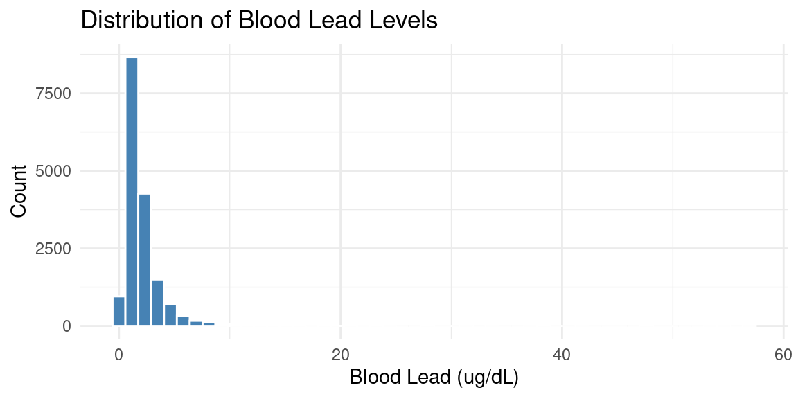
The distribution is right-skewed — most values are low with a long right tail.

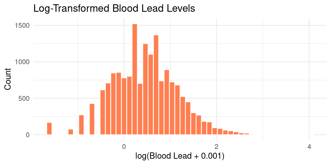
Why Log-Transform?

• Many exposure biomarkers have right-skewed distributions
• Log transformation makes the distribution more symmetric
• Improves linear model assumptions (normality of residuals)
• Common practice in environmental epidemiology

Log-Transforming Lead

NHData.train <- NHData.train %>%
  mutate(lead_logged = log(LBXBPB + 0.001))

ggplot(NHData.train, aes(x = lead_logged)) +
  geom_histogram(bins = 50, fill = "coral", color = "white") +
  labs(x = "log(Blood Lead + 0.001)", y = "Count",
       title = "Log-Transformed Blood Lead Levels") +
  theme_minimal()

Why Add 0.001?

• Some exposure values may be zero (below detection limit)
• \(\log(0) = -\infty\), so we add a small constant
• log(LBXBPB + 0.001) ensures all values are defined
• The constant (0.001) is small enough to not affect non-zero values substantially

Interpreting Log-Transformed Coefficients

# Rebuild design with updated data
dsn <- svydesign(ids = ~SDMVPSU, strata = ~SDMVSTRA,
                 weights = ~WTMEC2YR, nest = TRUE, data = NHData.train)
mod_log <- svyglm(LBXGLU ~ log(LBXBPB + 0.001), dsn)
tidy(mod_log) %>% kable(digits = 3) %>% kable_styling()

term	estimate	std.error	statistic	p.value
(Intercept)	98.294	0.628	156.535	0
log(LBXBPB + 0.001)	4.322	0.664	6.511	0

A 1-unit change in log(exposure) corresponds to a ~2.7-fold change in the raw exposure (since \(e^1 \approx 2.72\)).

Z-Score Standardization (Scaling)

Different exposures have different units (ug/dL, ng/mL, etc.). To compare across exposures:

\[z = \frac{x - \bar{x}}{s_x}\]

NHData.train <- NHData.train %>%
  mutate(lead_scaled = scale(log(LBXBPB + 0.001)))

NHData.train %>%
  summarize(
    raw_mean = mean(log(LBXBPB + 0.001), na.rm = TRUE),
    raw_sd = sd(log(LBXBPB + 0.001), na.rm = TRUE),
    scaled_mean = mean(lead_scaled, na.rm = TRUE),
    scaled_sd = sd(lead_scaled, na.rm = TRUE)
  ) %>%
  kable(digits = 3) %>% kable_styling()

raw_mean	raw_sd	scaled_mean	scaled_sd
0.46	0.713	0	1

Why Standardize?

After scaling:

• Mean = 0, SD = 1
• Coefficients represent the change in outcome per 1 SD change in the exposure
• All exposure associations are on the same scale
• Essential for comparing effect sizes across different exposures in ExWAS

The ExWAS Model

For each exposure \(E_j\), we fit:

\[\text{Phenotype} = \alpha + \beta_j \cdot \text{scale}(\log(E_j + 0.001)) + \gamma_1 \cdot \text{Age} + \gamma_2 \cdot \text{Sex} + \gamma_3 \cdot \text{Race} + \gamma_4 \cdot \text{Income} + \epsilon\]

• \(\beta_j\): effect of a 1 SD change in log-exposure on the phenotype
• Adjusted for confounders (age, sex, race, income)

Multiple Testing Problem

When testing \(m\) hypotheses simultaneously:

• At \(\alpha = 0.05\), we expect \(0.05 \times m\) false positives by chance
• With \(m = 160\) exposures: ~8 false positives expected
• We need multiple testing correction

Bonferroni Correction

The simplest approach — divide \(\alpha\) by the number of tests:

\[\alpha_{\text{Bonf}} = \frac{\alpha}{m} = \frac{0.05}{160} = 0.000313\]

• Controls the Family-Wise Error Rate (FWER)
• Probability of any false positive \(\leq \alpha\)
• Very conservative — may miss true associations

Benjamini-Hochberg FDR

A less conservative approach controlling the False Discovery Rate:

1. Rank p-values from smallest to largest: \(p_{(1)} \leq p_{(2)} \leq \cdots \leq p_{(m)}\)
2. Find the largest \(k\) such that \(p_{(k)} \leq \frac{k}{m} \cdot \alpha\)
3. Reject all hypotheses \(H_{(1)}, \ldots, H_{(k)}\)

• Controls the expected proportion of false discoveries among rejected hypotheses
• Less conservative than Bonferroni
• Preferred for ExWAS

FDR in R

# Simulated p-values for demonstration
set.seed(42)
pvalues <- c(runif(10, 0, 0.001), runif(150, 0, 1))  # 10 "real" + 150 null

# Bonferroni
bonf_adjusted <- p.adjust(pvalues, method = "bonferroni")

# Benjamini-Hochberg FDR
fdr_adjusted <- p.adjust(pvalues, method = "BH")

tibble(
  raw_p = sort(pvalues)[1:5],
  bonferroni = sort(bonf_adjusted)[1:5],
  fdr = sort(fdr_adjusted)[1:5]
) %>% kable(digits = 6) %>% kable_styling()

raw_p	bonferroni	fdr
0.000135	0.021547	0.01363
0.000239	0.038223	0.01363
0.000286	0.045782	0.01363
0.000519	0.083055	0.01363
0.000642	0.102679	0.01363

Bonferroni vs. FDR: Comparison

tibble(raw = sort(pvalues), bonf = sort(bonf_adjusted), fdr = sort(fdr_adjusted),
       rank = 1:length(pvalues)) %>%
  pivot_longer(cols = c(bonf, fdr), names_to = "method", values_to = "adjusted_p") %>%
  ggplot(aes(x = rank, y = adjusted_p, color = method)) +
  geom_point(alpha = 0.5) +
  geom_hline(yintercept = 0.05, linetype = "dashed") +
  scale_y_log10() +
  labs(x = "Rank", y = "Adjusted p-value (log scale)", title = "Bonferroni vs. FDR") +
  theme_minimal()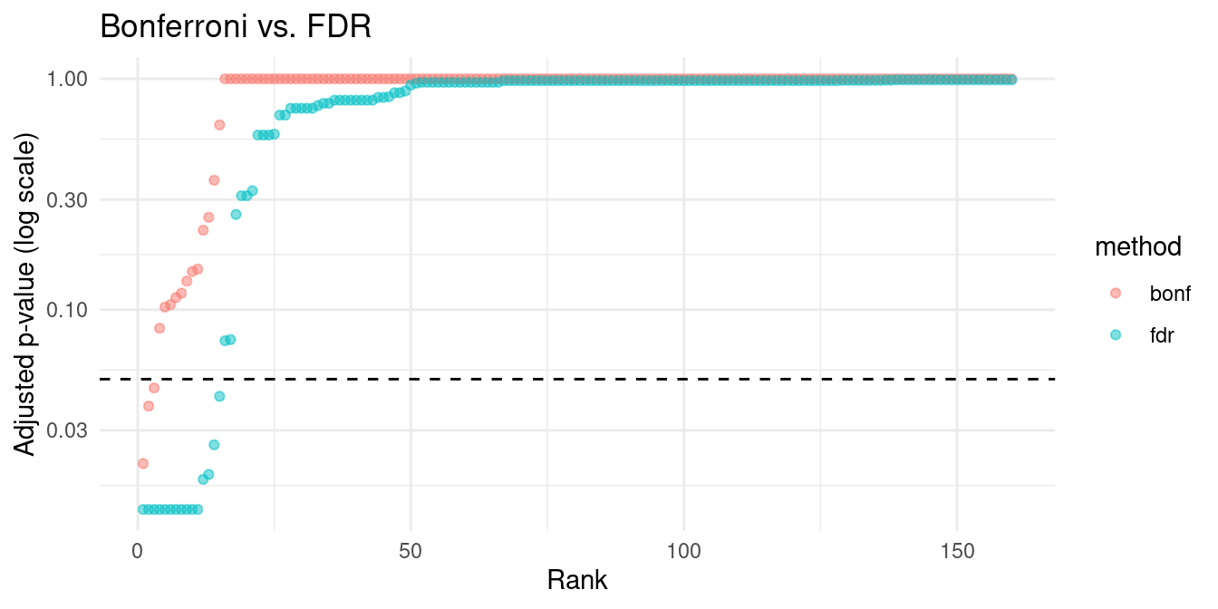

Confounding

A confounder C is a variable that:

1. Is associated with the exposure (E)
2. Is associated with the outcome (P)
3. Is NOT on the causal path from E to P

If we don’t adjust for C, the E-P association is biased.

Directed Acyclic Graphs (DAGs)

DAGs represent causal relationships:

     C
    / \
   v   v
   E   P

• C → E: confounder causes exposure level
• C → P: confounder causes phenotype
• Without adjusting for C, we see a spurious E-P association

Example: Age (C) affects both lead exposure (E) and BMI (P).

Adjusting for Confounders

In our ExWAS model, we adjust for:

Confounder	Why?
Age	Affects both exposure levels and health outcomes
Sex	Biological differences in metabolism and exposure
Race/Ethnicity	Sociostructural differences in exposure and health
Income (INDFMPIR)	Socioeconomic factors affect exposure and health

The Confounding Problem in ExWAS

A fundamental limitation of screening approaches like ExWAS:

Each exposure-phenotype pair has a different confounding structure — but we apply the same covariate set to all tests.

Lead → BMI:     confounders = age, SES, housing, occupation
Vitamin D → BMI: confounders = age, SES, physical activity, sun exposure
Cotinine → BMI:  confounders = age, SES, alcohol use, diet quality

There is no single DAG for the exposome — there are hundreds of DAGs, one per association.

Why This Matters

Using a “one-size-fits-all” covariate set means:

• Under-adjustment: missing a key confounder for some associations → false positives
• Over-adjustment: conditioning on a collider or descendant of the exposure → bias
• Heterogeneous bias: the direction and magnitude of bias differs across exposures

Example: Adjusting for BMI when testing diet → glucose may block a causal path (over-adjust), while failing to adjust for physical activity when testing vitamin D → BMI may leave confounding open (under-adjust).

Implications for ExWAS

This does not invalidate ExWAS — but it means:

1. ExWAS results are hypothesis-generating, not causal claims
2. The same covariate set is a practical necessity, not an ideal
3. Sensitivity analysis across multiple adjustment models (Module 4) helps assess robustness
4. Top hits should be followed up with exposure-specific DAGs and targeted analyses
5. Advanced methods can help mitigate this bias (Module 7)

R-Squared (\(R^2\))

\(R^2\) measures the proportion of variance in the outcome explained by the model:

\[R^2 = 1 - \frac{SS_{\text{res}}}{SS_{\text{tot}}}\]

mod_base <- lm(BMXBMI ~ RIDAGEYR + male +
               black + mexican + other_hispanic + other_eth +
               INDFMPIR, data = NHData.train)
glance(mod_base) %>%
  select(r.squared, adj.r.squared) %>%
  kable(digits = 4) %>% kable_styling()

r.squared	adj.r.squared
0.2343	0.234

Delta R-Squared (\(\Delta R^2\))

How much additional variance does the exposure explain beyond confounders?

\[\Delta R^2 = R^2_{\text{full}} - R^2_{\text{base}}\]

# Base model (confounders only)
r2_base <- summary(lm(BMXBMI ~ RIDAGEYR + male +
                      black + mexican + other_hispanic + other_eth +
                      INDFMPIR,
                      data = NHData.train))$r.squared

# Full model (confounders + exposure)
r2_full <- summary(lm(BMXBMI ~ scale(log(LBXBPB + 0.001)) +
                      RIDAGEYR + male +
                      black + mexican + other_hispanic + other_eth +
                      INDFMPIR,
                      data = NHData.train))$r.squared

tibble(r2_base = r2_base, r2_full = r2_full,
       delta_r2 = r2_full - r2_base) %>%
  kable(digits = 5) %>% kable_styling()

r2_base	r2_full	delta_r2
0.23431	0.25109	0.01678

Putting It Together: The ExWAS Pipeline

1. Set up survey design with svydesign()
2. For each exposure: log-transform and standardize
3. Fit svyglm() adjusting for confounders
4. Collect estimates, standard errors, p-values
5. Correct p-values with Benjamini-Hochberg FDR
6. Compare \(\Delta R^2\) across exposures
7. Replicate in independent dataset

Summary

• Survey-weighted methods (svydesign, svyglm) are essential for NHANES
• Log-transform skewed exposure distributions
• Standardize (Z-score) to compare effect sizes across exposures
• Multiple testing correction: FDR preferred over Bonferroni for ExWAS
• Confounders must be identified and adjusted for (use DAGs)
• Confounders differ per association — a major limitation of one-size-fits-all screening
• \(\Delta R^2\) quantifies the unique contribution of each exposure

What’s Next?

Module 4: The nhanespewas Package

• Installing and connecting to the nhanespewas database
• Exploring exposure and phenotype catalogs
• Understanding adjustment models
• First ExWAS with pe_flex_adjust()

Supported By

This course is supported by the National Institutes of Health (NIH):

• National Institute of Environmental Health Sciences (NIEHS): R01ES032470, U24ES036819
• National Institute of Diabetes and Digestive and Kidney Diseases (NIDDK): R01DK137993